

Dynamic Programming

The term dynamic programming (DP) refers to a collection of algorithms that can be used to compute optimal policies given a perfect model of the environment as a Markov decision process (MDP).

The key idea of DP, and of reinforcement learning generally, is the use of value functions to organize and structure the search for good policies.

In the dynamic programming setting, the agent has full knowledge of the MDP. (This is much easier than the reinforcement learning setting, where the agent initially knows nothing about how the environment decides state and reward and must learn entirely from interaction how to select actions.)

An Iterative Method

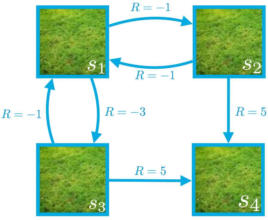
In order to obtain the state-value function $v_\pi$ corresponding to a policy $\pi$, we need to solve the system of equations corresponding to the Bellman expectation equation for $v_\pi$.

Notes on the Bellman Expectation Equation

for state $s_1$, we saw that:

$$v_\pi(s_1) = \frac{1}{2}(-1 + v_\pi(s_2)) + \frac{1}{2}(-3 + v_\pi(s_3))$$

We mentioned that this equation follows directly from the Bellman expectation equation for $v_\pi$

$$v_\pi(s) = \text{} \mathbb{E}_\pi[R_{t+1} + \gamma v_\pi(S_{t+1}) | S_t=s] = \sum_{a \in \mathcal{A}(s)}\pi(a|s)\sum_{s' \in \mathcal{S}, r\in\mathcal{R}}p(s',r|s,a)(r + \gamma v_\pi(s'))$$

(The Bellman expectation equation for $v_\pi$)

In order to see this, we can begin by looking at what the Bellman expectation equation tells us about the value of state $s_1$ (where we just need to plug in s_1 for state $s$).

$$v_\pi(s_1) = \sum_{a \in \mathcal{A}(s_1)}\pi(a|s_1)\sum_{s' \in \mathcal{S}, r\in\mathcal{R}}p(s',r|s_1,a)(r + \gamma v_\pi(s'))$$

Then, it's possible to derive the equation for state $s_1$ by using the following:

• $\mathcal{A}(s_1=\{ \text{down}, \text{right} \}$ (When in state s_1, the agent only has two potential actions: down or right.)
• $\pi({down}|s_1) = \pi(\text{right}|s_1) = \frac{1}{2}$ (We are currently examining the policy where the agent goes down with 50% probability and right with 50% probability when in state $s_1$.)
• $p(s_3,-3|s_1,\text{down}) = 1 (\text{and } p(s',r|s_1,\text{down}) = 0 \text{ if } s'\neq s_3 \text{ or } r\neq -3)$ (If the agent chooses to go down in state $s_1$ then with 100% probability, the next state is $s_3$, and the agent receives a reward of -3.)
• $p(s_2,-1|s_1,\text{right}) = 1 (\text{and } p(s',r|s_1,\text{right}) = 0 \text{ if } s'\neq s_2 \text{ or } r\neq -1)$ (If the agent chooses to go right in state $s_1$, then with 100% probability, the next state is $s_2$, and the agent receives a reward of -1.)
• $\gamma = 1$ (We chose to set the discount rate to 1 in this gridworld example.)

Notes on Solving the System of Equations

This example serves to illustrate the fact that it is possible to directly solve the system of equations given by the Bellman expectation equation for $v_\pi$ However, in practice, and especially for much larger Markov decision processes (MDPs), we will instead use an iterative solution approach.

You can directly solve the system of equations:

$v_\pi(s_1) = \frac{1}{2}(-1 + v_\pi(s_2)) + \frac{1}{2}(-3 + v_\pi(s_3))$

$v_\pi(s_2) = \frac{1}{2}(-1 + v_\pi(s_1)) + \frac{1}{2}(5 + v_\pi(s_4))$

$v_\pi(s_3) = \frac{1}{2}(-1 + v_\pi(s_1)) + \frac{1}{2}(5 + v_\pi(s_4))$

$v_\pi(s_4) = 0$

Since the equations for $v_\pi(s_2)$ and $v_\pi(s_3)$ are identical, we must have that $v_\pi(s_2) = v_\pi(s_3)$

Thus, the equations for $v_\pi(s_1)$ and $v_\pi(s_2)$ can be changed to:

$v_\pi(s_1) = \frac{1}{2}(-1 + v_\pi(s_2)) + \frac{1}{2}(-3 + v_\pi(s_2)) = -2 + v_\pi(s_2)$

$v_\pi(s_2) = \frac{1}{2}(-1 + v_\pi(s_1)) + \frac{1}{2}(5 + 0) = 2 + \frac{1}{2}v_\pi(s_1)$

Combining the two latest equations yields

$v_\pi(s_1) = -2 + 2 + \frac{1}{2}v_\pi(s_1) = \frac{1}{2}v_\pi(s_1)$

which implies $v_\pi(s_1)=0$ Furthermore, $v_\pi(s_3) = v_\pi(s_2) = 2 + \frac{1}{2}v_\pi(s_1) = 2 + 0 = 2$

Thus, the state-value function is given by:

$v_\pi(s_1) = 0$

$v_\pi(s_2) = 2$

$v_\pi(s_3) = 2$

$v_\pi(s_4) = 0$

we have discussed how an agent might obtain the state-value function $v_\pi$ corresponding to a policy $\pi$.

In the dynamic programming setting, the agent has full knowledge of the Markov decision process (MDP). In this case, it's possible to use the one-step dynamics $p(s',r|s,a)$ of the MDP to obtain a system of equations corresponding to the Bellman expectation equation for $v_\pi$.

In order to obtain the state-value function, we need only solve the system of equations.

While it is always possible to directly solve the system, we will instead use an iterative solution approach.

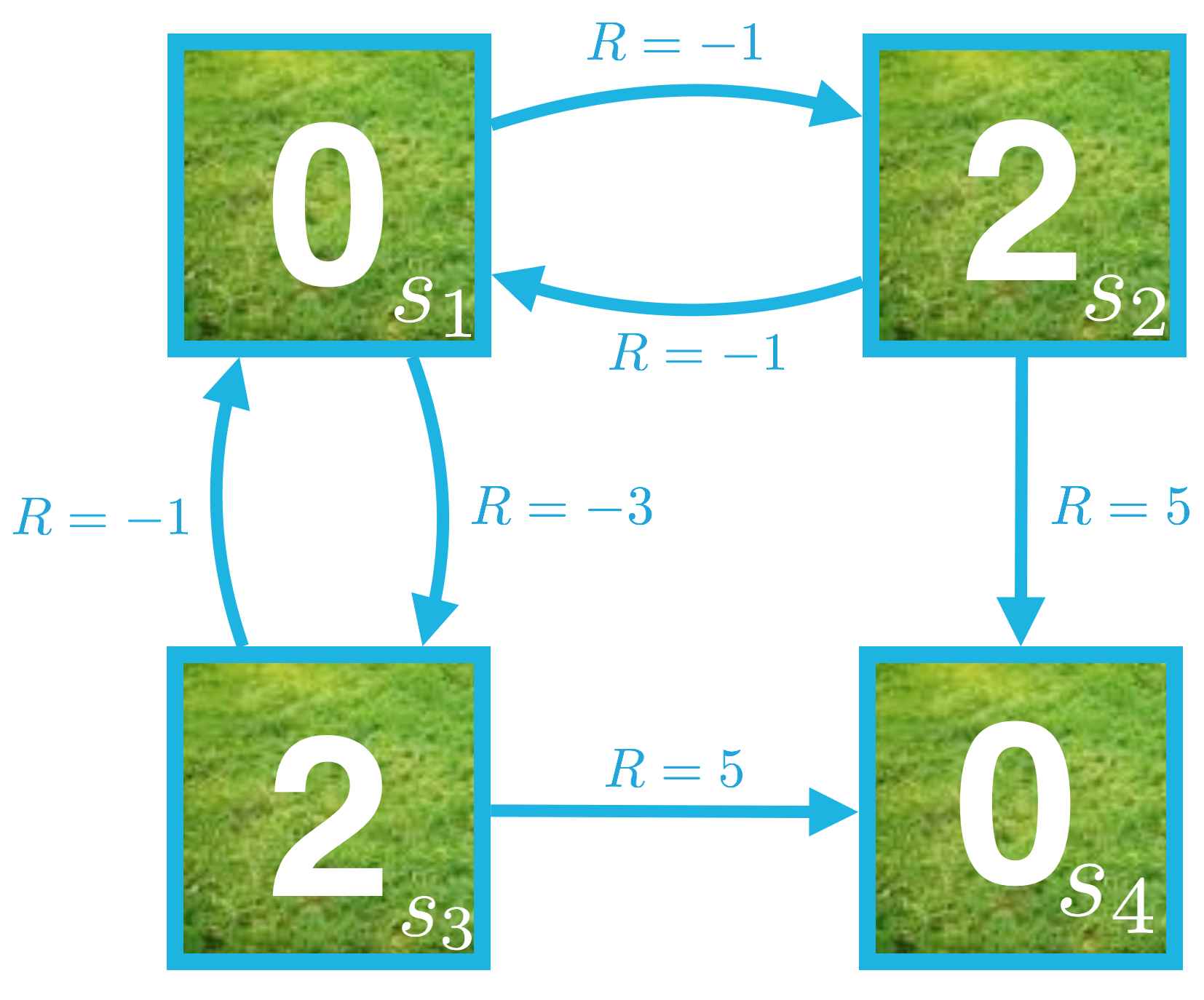
The iterative method begins with an initial guess for the value of each state. In particular, we began by assuming that the value of each state was zero.

Then, we looped over the state space and amended the estimate for the state-value function through applying successive update equations.

Recall that $V$ denotes the most recent guess for the state-value function, and the update equations are:

$$V(s_1) \leftarrow \frac{1}{2}(-1 + V(s_2)) + \frac{1}{2}(-3 + V(s_3))$$

$$V(s_2) \leftarrow \frac{1}{2}(-1 + V(s_1)) + \frac{1}{2}(5)$$

$$V(s_3) \leftarrow \frac{1}{2}(-1 + V(s_1)) + \frac{1}{2}(5)$$

The state-value function for the equiprobable random policy is visualized below:

Iterative Policy Evaluation

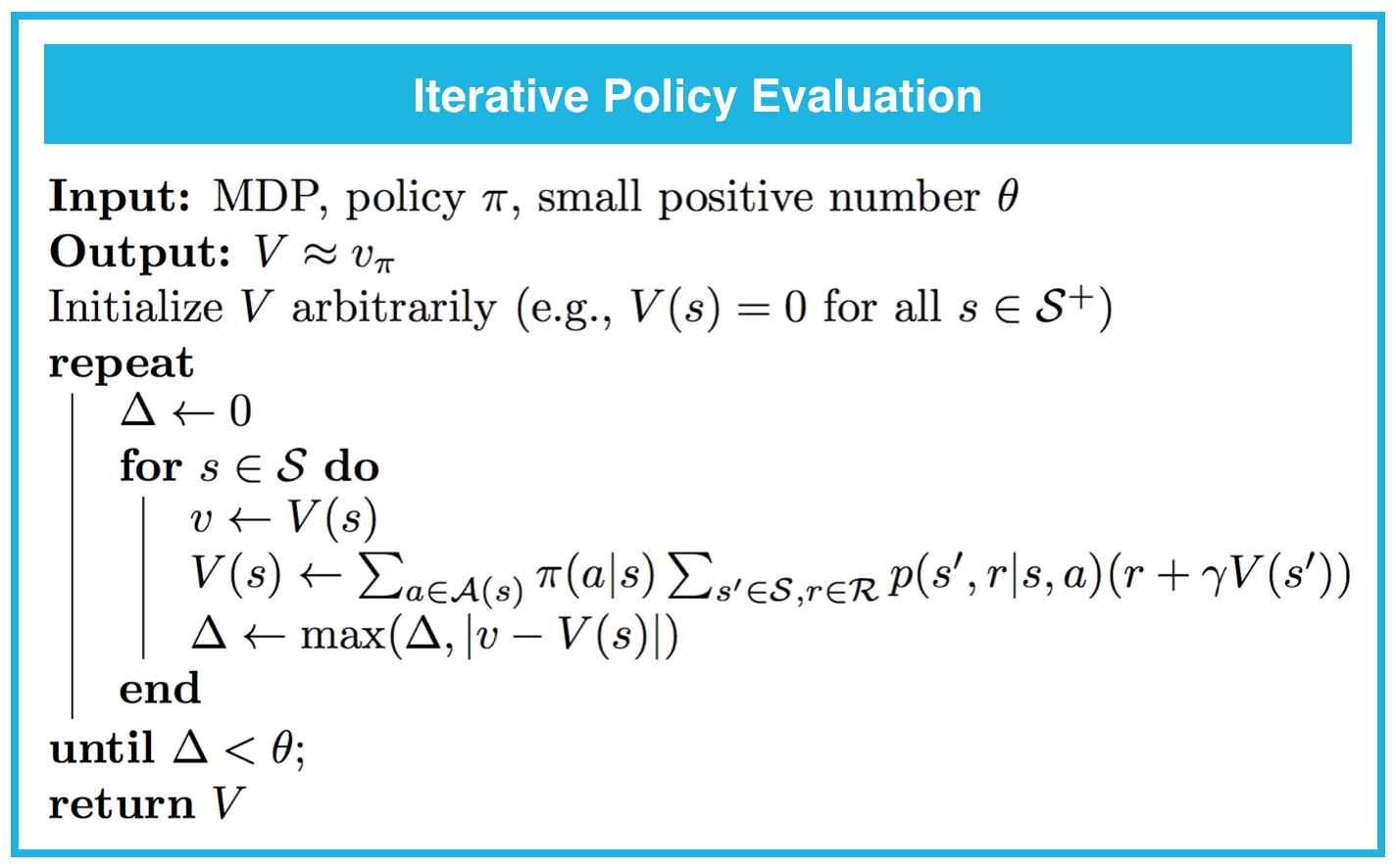
Note that policy evaluation is guaranteed to converge to the state-value function $v_\pi$ corresponding to a policy $\pi$, as long as $v_\pi(s)$ is finite for each state $s\in\mathcal{S}$. For a finite Markov decision process (MDP), this is guaranteed as long as either:

• $\gamma < 1$, or
• if the agent starts in any state $s\in\mathcal{S}$, it is guaranteed to eventually reach a terminal state if it follows policy $\pi$.

Action Values

Use the simple gridworld to practice converting a state-value function $v_\pi$ to an action-value function $q_\pi$

Image below corresponds to the action-value function for the same policy.

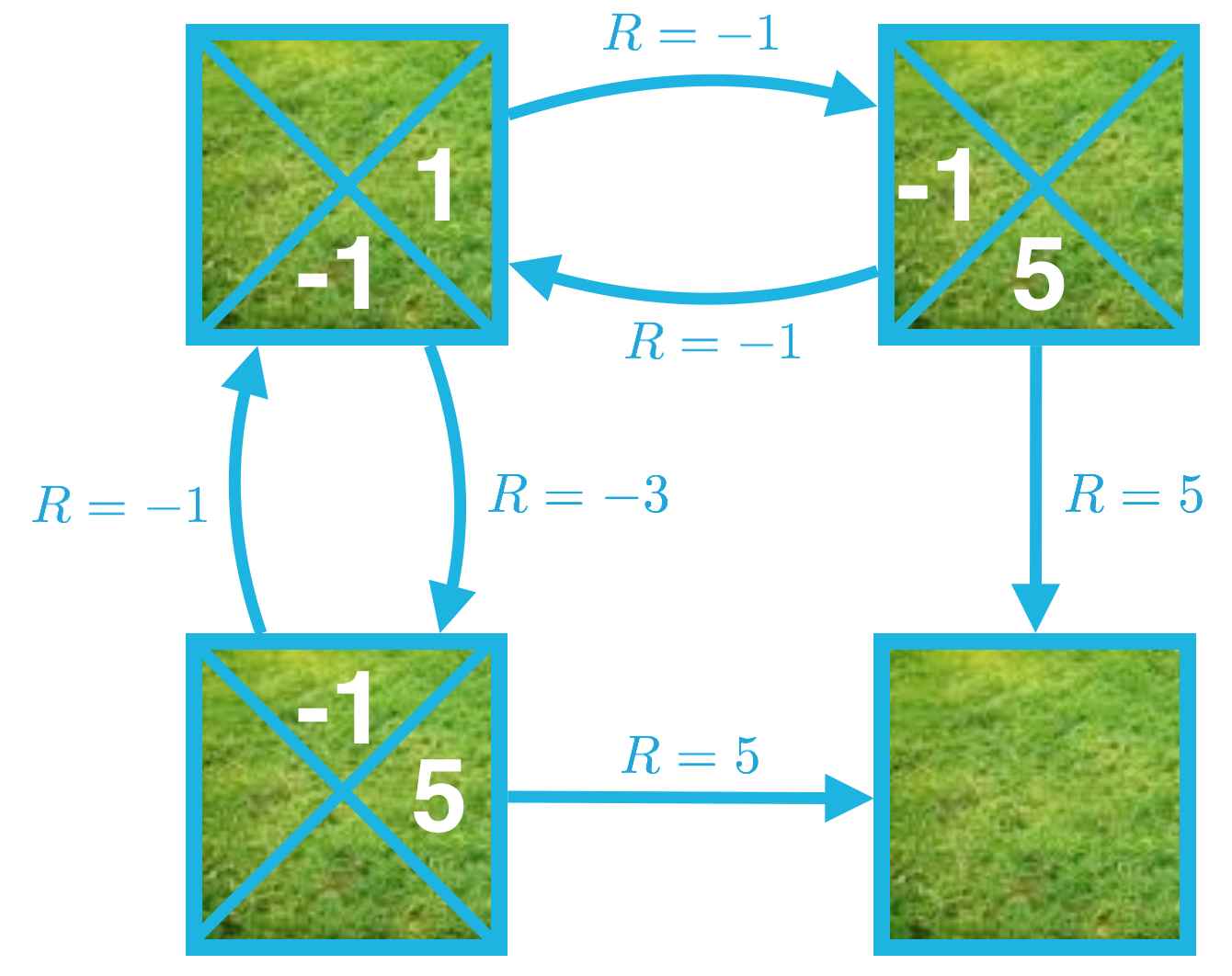
As an example, consider $q_\pi(s_1, \text{right})$. This action value can be calculated as

$q_\pi(s_1, \text{right}) = -1 + v_\pi(s_2) = -1 + 2 = 1$

where we just use the fact that we can express the value of the state-action pair $s_1, \text{right}$ as the sum of two quantities:

• the immediate reward after moving right and landing on state $s_2$
• the cumulative reward obtained if the agent begins in state $s_2$ and follows the policy.

For More Complex Environments

In this simple gridworld example, the environment is deterministic. In other words, after the agent selects an action, the next state and reward are 100% guaranteed and non-random. For deterministic environments, $p(s',r|s,a) \in {0,1} \text{ for all } s', r, s, a$

In this case, when the agent is in state s and takes action $a$, the next state $s'$ and reward $r$ can be predicted with certainty, and we must have $q_\pi(s,a) = r + \gamma v_\pi(s')$

In general, the environment need not be deterministic, and instead may be stochastic. This is the default behavior of the FrozenLake environment; in this case, once the agent selects an action, the next state and reward cannot be predicted with certainty and instead are random draws from a (conditional) probability distribution $p(s',r|s,a)$

In this case, when the agent is in state $s$ and takes action $a$, the probability of each possible next state $s'$ and reward $r$ is given by $p(s',r|s,a)$. In this case, we must have $q_\pi(s,a) = \sum_{s'\in\mathcal{S}^+, r\in\mathcal{R}}p(s',r|s,a)(r+\gamma v_\pi(s'))$, where we take the expected value of the sum $r + \gamma v_\pi(s')$

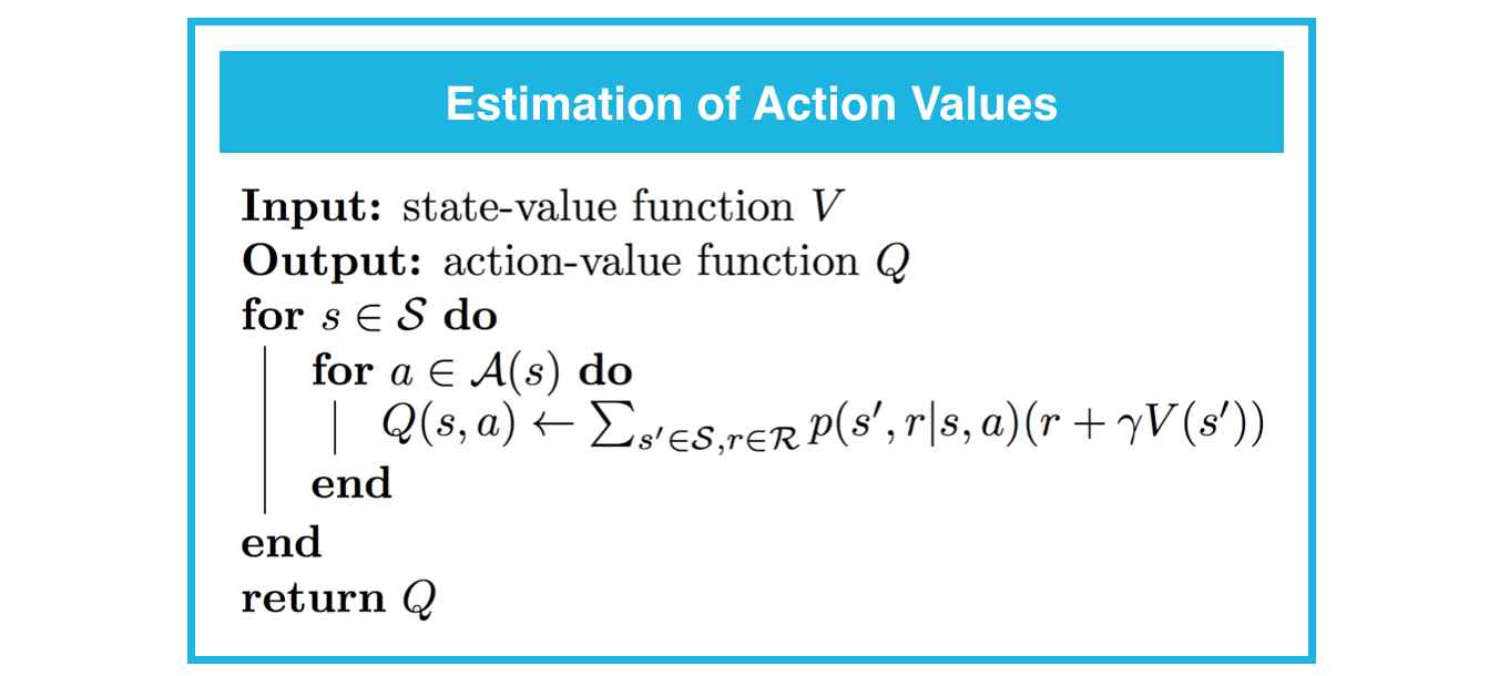
Estimation of Action Values

Write an algorithm that accepts an estimate $V$ of the state-value function $v_\pi$ along with the one-step dynamics of the MDP $p(s',r|s,a)$ and returns an estimate $Q$ the action-value function $q_\pi$

Use the one-step dynamics $p(s',r|s,a)$ of MDP to obtain $q_\pi$ from $v_\pi$. Namely,

$q_\pi(s,a) = \sum_{s'\in\mathcal{S}^+, r\in\mathcal{R}}p(s',r|s,a)(r+\gamma v_\pi(s'))$ holds for all $s\in\mathcal{S} \text{ and } a\in\mathcal{A}(s)$.

Policy Improvement

Our reason for computing the value function for a policy is to help find better policies. Suppose we have determined the value function $v_\pi$ for an arbitrary deterministic policy $\pi$. For some state $s$ we would like to know whether or not we should change the policy to deterministically choose an action $a \neq \pi(s)$.

Implementation

It is possible to construct an improved (or equivalent) policy $\pi'$, where $\pi'\geq\pi$

For each state $s\in\mathcal{S}$, you need to select the action that maximizes the action-value function estimate. In other words,

$\pi'(s)=\arg\max_{a\in\mathcal{A}(s)}Q(s,a)$ for all $s\in\mathcal{S}$.

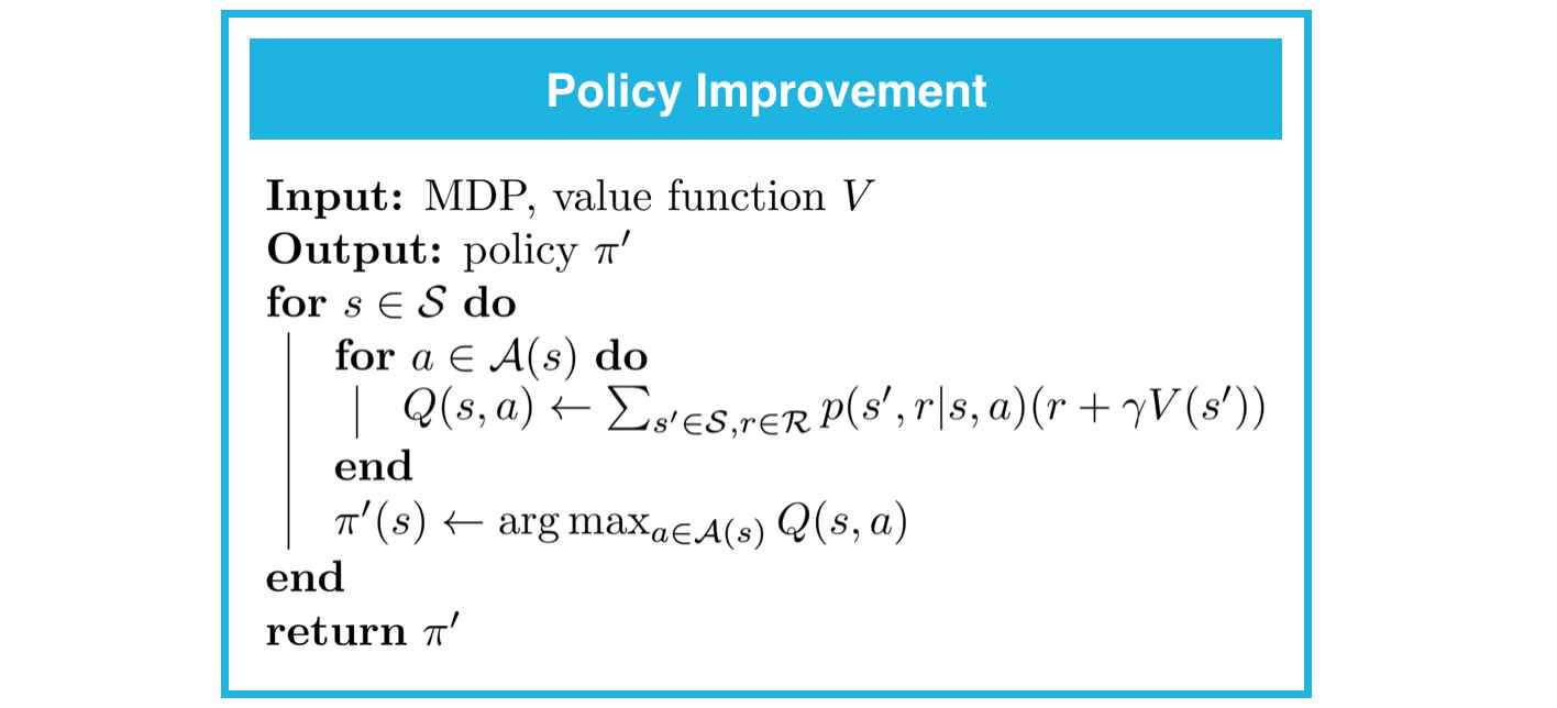
In the event that there is some state $s\in\mathcal{S}$ for which $\arg\max_{a\in\mathcal{A}(s)}$ is not unique, there is some flexibility in how the improved policy $\pi'$ is constructed.

In fact, as long as the policy $\pi'$ satisfies for each $s\in\mathcal{S}$ and $a\in\mathcal{A}(s)$:

$\pi'(a|s)=0 \text{ if a }\notin \arg\max_{a'\in\mathcal{A}(s)}Q(s,a')$

It is an improved policy. In other words, any policy that (for each state) assigns zero probability to the actions that do not maximize the action-value function estimate (for that state) is an improved policy.

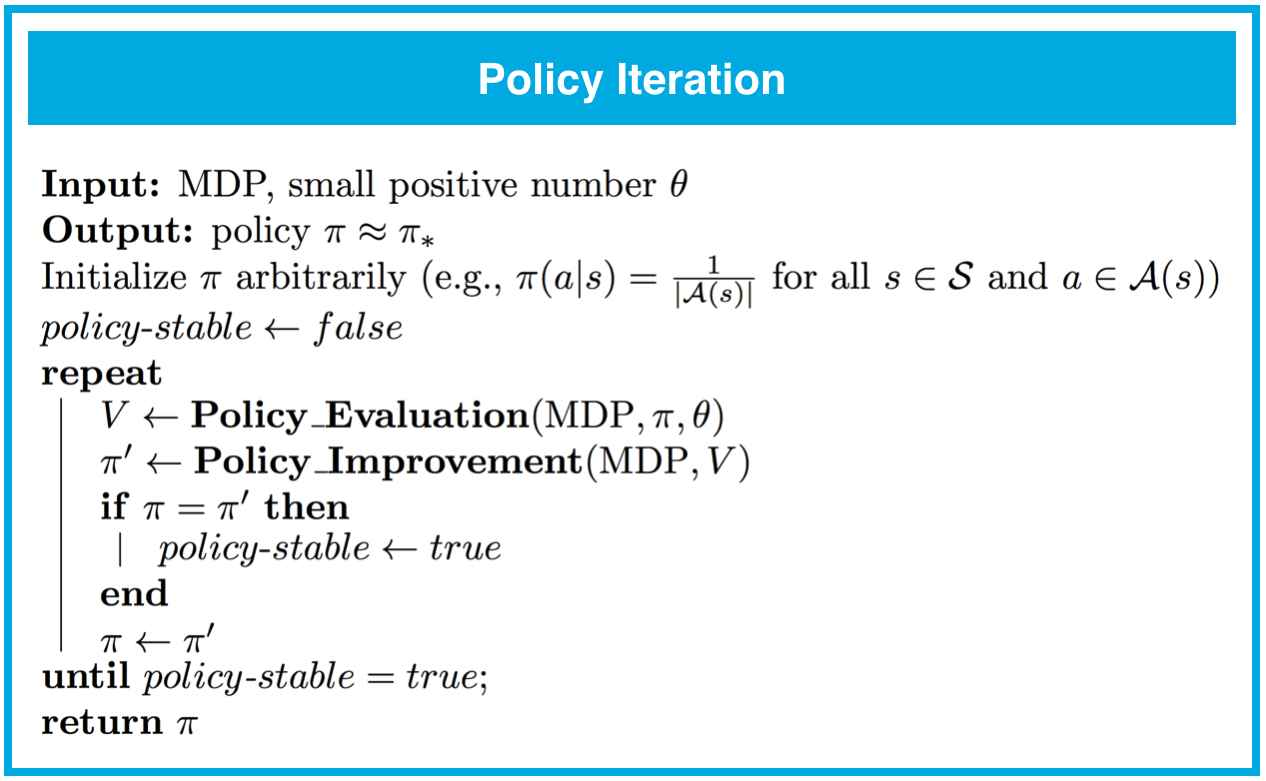
Policy Iteration

This way of finding an optimal policy is called policy iteration.

Policy iteration is guaranteed to find the optimal policy for any finite Markov decision process (MDP) in a finite number of iterations.

Value Iteration

One drawback to policy iteration is that each of its iterations involves policy evaluation, which may itself be a protracted iterative computation requiring multiple sweeps through the state set. If policy evaluation is done iteratively, then convergence exactly to $v_\pi$ occurs only in the limit.

In fact, the policy evaluation step of policy iteration can be truncated in several ways without losing the convergence guarantees of policy iteration. One important special case is when policy evaluation is stopped after just one sweep (one update of each state). This algorithm is called value iteration.

In this algorithm, each sweep over the state space effectively performs both policy evaluation and policy improvement. Value iteration is guaranteed to find the optimal policy $\pi_*$ for any finite MDP.

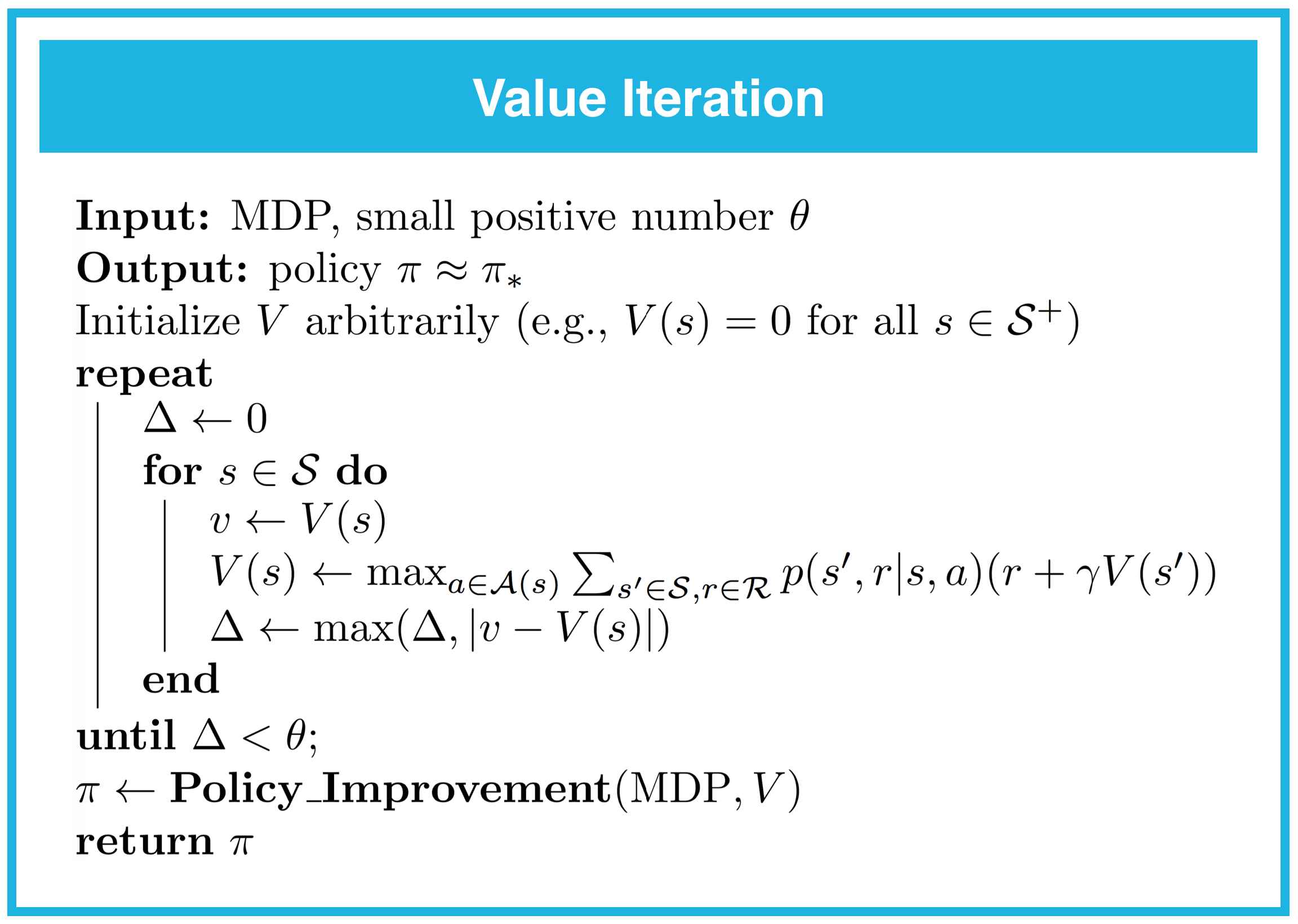
Note that the stopping criterion is satisfied when the difference between successive value function estimates is sufficiently small. In particular, the loop terminates if the difference is less than $\theta$ for each state. And, the closer we want the final value function estimate to be to the optimal value function, the smaller we need to set the value of $\theta$.

note that in the case of the FrozenLake environment, values around 1e-8 seem to work reasonably well.