

Monte Carlo Methods

Monte Carlo methods require only experience - sample sequences of states, actions, and rewards from actual or simulated interaction with an environment but no complete knowledge of environment.

Only on the completion of an episode are value estimates and policies changed. Monte Carlo methods can thus be incremental in an episode-by-episode sense, but not in a step-by-step (online) sense.

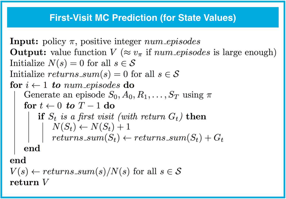
The first-visit MC method estimates $v_\pi(s)$ as the average of the returns following first visits to $s$, whereas the every-visit MC method averages the returns following all visits to $s$.

• Every-visit MC is biased, whereas first-visit MC is unbiased.
• Initially, every-visit MC has lower mean squared error (MSE), but as more episodes are collected, first-visit MC attains better MSE.

Both the first-visit and every-visit method are guaranteed to converge to the true value function, as the number of visits to each state approaches infinity.

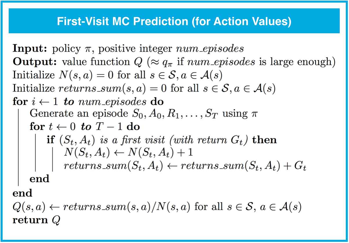
MC Prediction (Action Values)

If a model is not available, then it is particularly useful to estimate action values (the values of state–action pairs) rather than state values.

With a model, state values alone are sufficient to determine a policy; one simply looks ahead one step and chooses whichever action leads to the best combination of reward and next state.

We won't use MC prediction to estimate the action-values corresponding to a deterministic policy; this is because many state-action pairs will never be visited (since a deterministic policy always chooses the same action from each state). Instead, so that convergence is guaranteed, we will only estimate action-value functions corresponding to policies where each action has a nonzero probability of being selected from each state.

Exploration-Exploitation Dilemma

At every time step, when the agent selects an action, it bases its decision on past experience with the environment. And, towards minimizing the number of episodes needed to solve environments in OpenAI Gym, our first instinct could be to devise a strategy where the agent always selects the action that it believes (based on its past experience) will maximize return. With this in mind, the agent could follow the policy that is greedy with respect to the action-value function estimate. We examined this approach in a previous video and saw that it can easily lead to convergence to a sub-optimal policy.

To see why this is the case, note that in early episodes, the agent's knowledge is quite limited (and potentially flawed). So, it is highly likely that actions estimated to be non-greedy by the agent are in fact better than the estimated greedy action

With this in mind, a successful RL agent cannot act greedily at every time step (that is, it cannot always exploit its knowledge); instead, in order to discover the optimal policy, it has to continue to refine the estimated return for all state-action pairs (in other words, it has to continue to explore the range of possibilities by visiting every state-action pair). That said, the agent should always act somewhat greedily, towards its goal of maximizing return as quickly as possible. This motivated the idea of an $\epsilon$-greedy policy.

We refer to the need to balance these two competing requirements as the Exploration-Exploitation Dilemma. One potential solution to this dilemma is implemented by gradually modifying the value of $\epsilon$ when constructing $\epsilon$-greedy policies.

Setting the Value of $\epsilon$, in Theory

It makes sense for the agent to begin its interaction with the environment by favoring exploration over exploitation. After all, when the agent knows relatively little about the environment's dynamics, it should distrust its limited knowledge and explore, or try out various strategies for maximizing return. With this in mind, the best starting policy is the equiprobable random policy, as it is equally likely to explore all possible actions from each state. You discovered in the previous quiz that setting $\epsilon = 1$ yields an $\epsilon$-greedy policy that is equivalent to the equiprobable random policy.

At later time steps, it makes sense to favor exploitation over exploration, where the policy gradually becomes more greedy with respect to the action-value function estimate. After all, the more the agent interacts with the environment, the more it can trust its estimated action-value function. You discovered in the previous quiz that setting $\epsilon = 0$ yields the greedy policy (or, the policy that most favors exploitation over exploration).

Thankfully, this strategy (of initially favoring exploration over exploitation, and then gradually preferring exploitation over exploration) can be demonstrated to be optimal.

GLIE

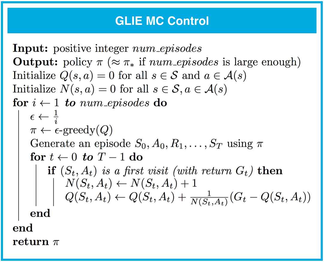
In order to guarantee that MC control converges to the optimal policy $\pi_*$, we need to ensure that two conditions are met. We refer to these conditions as Greedy in the Limit with Infinite Exploration (GLIE). In particular, if:

• every state-action pair $s$, $a$ (for all $s\in\mathcal{S} \text{ and } a\in\mathcal{A}(s)$) is visited infinitely many times, and
• the policy converges to a policy that is greedy with respect to the action-value function estimate $Q$,

then MC control is guaranteed to converge to the optimal policy (in the limit as the algorithm is run for infinitely many episodes). These conditions ensure that:

• the agent continues to explore for all time steps, and
• the agent gradually exploits more (and explores less).

One way to satisfy these conditions is to modify the value of $\epsilon$ when specifying an $\epsilon$-greedy policy. In particular, let $\epsilon_i$ correspond to the $i$-th time step. Then, both of these conditions are met if:

• $epsilon_i\gt0$ for all time steps $i$, and
• $\epsilon_i$ decays to zero in the limit as the time step $i$ approaches infinity (that is, $\lim_{i\to\infty} \epsilon_i = 0$)

For example, to ensure convergence to the optimal policy, we could set $\epsilon_i = \frac{1}{i}$ (You are encouraged to verify that $\epsilon_i \gt 0$ for all $i$, and $\lim_{i\to\infty} \epsilon_i = 0$

Setting the Value of $\epsilon$, in Practice

As you read in the above section, in order to guarantee convergence, we must let $\epsilon_i$ decay in accordance with the GLIE conditions. But sometimes "guaranteed convergence" isn't good enough in practice, since this really doesn't tell you how long you have to wait! It is possible that you could need trillions of episodes to recover the optimal policy, for instance, and the "guaranteed convergence" would still be accurate!

Even though convergence is not guaranteed by the mathematics, you can often get better results by either: - using fixed $\epsilon$, or - letting $\epsilon_i$ decay to a small positive number, like 0.1.

This is because one has to be very careful with setting the decay rate for $\epsilon$; letting it get too small too fast can be disastrous. If you get late in training and $\epsilon$ is really small, you pretty much want the agent to have already converged to the optimal policy, as it will take way too long otherwise for it to test out new actions!

MC Control: GLIE

MC Control: Constant-alpha

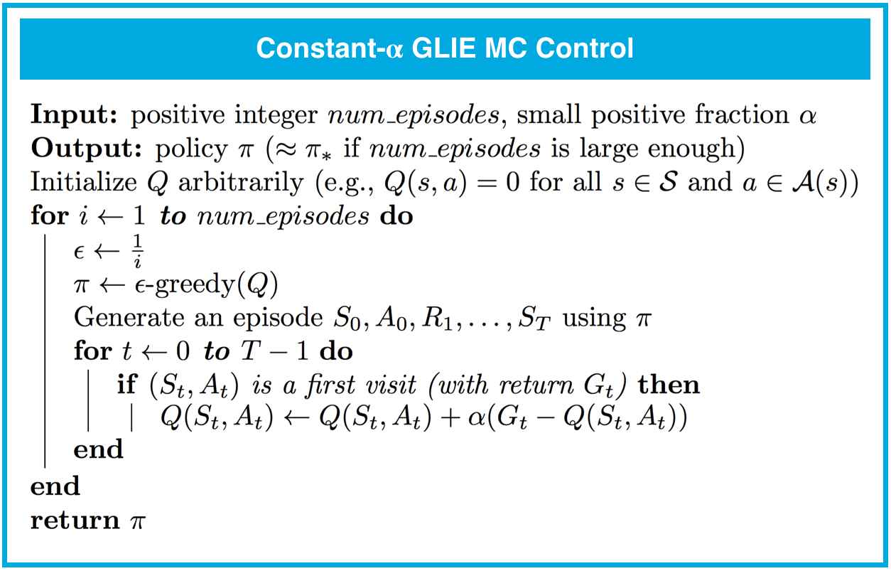
When we adapted running_mean algorithm for Monte Carlo control in the following concept (MC Control: Policy Evaluation), the sequence $(x_1, x_2, \ldots, x_n)$ corresponded to returns obtained after visiting the same state-action pair.

That said, the sampled returns (for the same state-action pair) likely corresponds to many different policies. This is because the control algorithm proceeds as a sequence of alternating evaluation and improvement steps, where the policy is improved after every episode of interaction. In particular, we discussed that returns sampled at later time steps likely correspond to policies that are more optimal.

With this in mind, it made sense to amend the policy evaluation step to instead use a constant step size, which we denoted by $\alpha$. This ensures that the agent primarily considers the most recently sampled returns when estimating the action-values and gradually forgets about returns in the distant past.

Setting the Value of $\alpha$

forgetful_mean function is closely related to the Evaluation step in constant-$\alpha$ MC control.

How to set the value of $\alpha$ when implementing constant-$\alpha$ MC control:

• You should always set the value for $\alpha$ to a number greater than zero and less than (or equal to) one.
  • If $\alpha=0$, then the action-value function estimate is never updated by the agent.
  • If $\alpha=1$, then the final value estimate for each state-action pair is always equal to the last return that was experienced by the agent (after visiting the pair).
• Smaller values for $\alpha$ encourage the agent to consider a longer history of returns when calculating the action-value function estimate. Increasing the value of $\alpha$ ensures that the agent focuses more on the most recently sampled returns.

Note that it is also possible to verify the above facts by slightly rewriting the update step as follows:

$Q(S_t,A_t) \leftarrow (1-\alpha) Q(S_t,A_t)+\alpha G_t$

where it is now more obvious that \alphaα controls how much the agent trusts the most recent return $G_t$ over the estimate $Q(S_t,A_t)$ constructed by considering all past returns.

IMPORTANT NOTE: It is important to mention that when implementing constant-$\alpha$ MC control, you must be careful to not set the value of $\alpha$ too close to 1. This is because very large values can keep the algorithm from converging to the optimal policy $\pi_*$. However, you must also be careful to not set the value of $\alpha$ too low, as this can result in an agent who learns too slowly. The best value of $\alpha$ for your implementation will greatly depend on your environment and is best gauged through trial-and-error.